
Labs using R: UBC Edition
Lab
1. Introduction to R
This lab is part of a series designed for BIOL 300, based on The Analysis of Biological Data. The rest of the labs can be found here.
Learning outcomes
Learning how to start with R and RStudio
Use functions in R
Write and save an R script
Data, R scripts, and other resources for these labs can be downloaded from here as a .zip file. Please open the ABDLabs folder created by the .zip file in a location on your computer that you can come back to use repeatedly.
Learning the tools
What is R?
R is a computer program that allows an extraordinary range of statistical calculations. It is a free program, mainly written by voluntary contributions from statisticians around the world. R is available on most operating systems, including Windows, Mac OS, and Linux.
R can make graphics and do statistical calculations. It is also a full-fledged computing language. In this series of labs, we will only scratch the surface of what R can do.
What is RStudio?
RStudio is a separate program, also free, that provides a more elegant front end for R. RStudio allows you to easily organize separate windows for R commands, graphic, help, etc. in one place.
If your computer does not already have a version of R and RStudio installed, look at the instructions for getting set up.
Getting started
If you haven’t done so already, download the folder called ABDLabs. Inside this folder are all the data sets
you will need for these labs. Also, there is a file in that folder
called ABDLabs.Rproj. Double-click on this file to start R and
RStudio. If you start R from this file, it will automatically
load some packages that will add some useful functionality, and it will
tell R to look for files inside the ABDLabs folder. Both of
these will let you skip some steps later.
You can also start R and Rstudio directly from the RStudio application. The icon for the application should look something like this:
![]()
When you start RStudio, it will automatically start R as well. You run R inside RStudio.
After you have started RStudio, you should see a new window with a menu bar at the top and three main sections. One of the sections is called the “Console” – this is where you type commands to give instructions to R and typically where you see R’s answers to you.
Another important corner of this window can show a variety of information. Most importantly to us, this is where graphics will appear, under the tab marked “Plots”.
The Console
When you start RStudio, you’ll see a corner of the window called the “Console”. By the default the console window is in the bottom left of the Rstudio screen.
You can type commands in this window where there is a prompt (which
will look like a > sign at the bottom of the window).
The Console has to be the selected window. (Clicking anywhere in the
Console selects it.)
The > prompt is R’s way of inviting you to give it
instructions. You communicate with R by typing commands after the
> prompt.
Type “2 + 2” at the > prompt, and
hit return. You’ll see that R can work like a calculator (among its many
other powers). It will give you the answer, 4, and it will label that
answer with [1] to indicate that it is the first element in
the answer. (This is sort of annoying when the answers are simple like
this, but can be very valuable when the answers become more
complex.)
In these labs, the input will show up in a gray box and the output, if any, will follow in a white box.
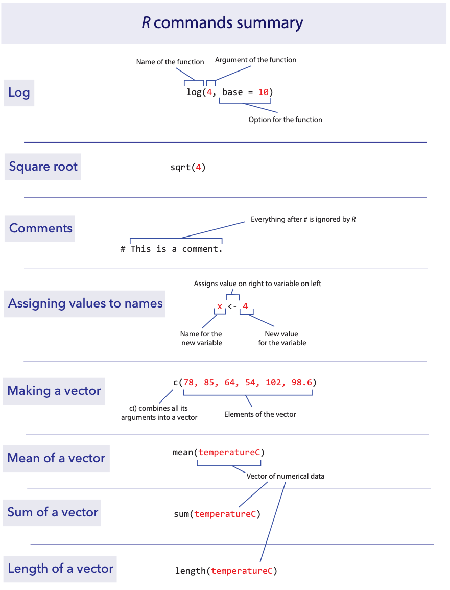
## [1] 4log()
You can use a wide variety of math functions to make calculations
here, e.g., log() calculates the log of a number:
## [1] 3.73767(By default, this gives the natural log with base e.)
Parentheses are used both as a way to group elements of the
calculation and also as a way to denote the arguments of functions. (The
“arguments” of a function are the set of values given to it as input.)
For example, log(3) is applying the function
log() to the argument 3.
sqrt()
Another mathematical function that often comes in handy is the square
root function, sqrt(). For example, the square root of 4
is:
## [1] 2To calculate a value with an exponent, use the ^ symbol.
For example 43 is written as:
## [1] 64Of course, many math functions can be combined to give an almost infinite possibility of mathematical expressions. For example,
\[\frac{1}{\sqrt{2\pi (3.1)^2}} e^{-\frac{(12-10.7)^2}{2(3.1) }}\]
can be calculated with
## [1] 0.09798692Writing and saving R scripts
You should keep a record of all commands used, along with copious
notes, so that weeks or years later you can retrace the steps of your
earlier analysis. An .R script provides a convenient way to
do this.
In RStudio, you can create an .R script file which
contains R commands that can be reloaded and used at a later date. Under
the menu at the top, choose File → New File → R Script.
This will create a new section in RStudio with the temporary name
“Untitled1” (or similar). You can copy and paste any commands that you
want from the Console, or type directly here. (When you copy and paste,
it’s better to not include the > prompt in the
script.)
To keep this script for later, just hit Save under the File menu. In the future you can open this file to have those commands available for use again.
It is best to type all your commands in the script window and run them from there, rather than typing directly into the console. This lets you save a record of your session so that you can more easily re-create what you have done later.
Functions
Most of the work in R is done by functions. A function has a name and
one or more arguments. For example, log(4) is a function
that calculates the log in base e for the value 4 given as input.
Sometimes functions have optional input arguments. For the function
log(), for example, we can specify the optional input
argument base to tell the function what base to use for the
logarithm. If we don’t specify the base variable, it has a default value
of base = e. To get a log in base 10, for example, we would
use:
## [1] 0.60206Defining objects
In R, we can store information of various sorts by assigning them to
objects. For example, if we want to create a object called
x and give it a value of 4, we would write
The middle bit of this: <-, a less than sign and a
hyphen typed together to make something that looks a little like a
left-facing arrow, tells R to assign the value on the right to the
object on the left. After running the command above, whenever we use
x in a command it would be replaced by its value 4. For
example, if we add 3 to x, we would expect to get 7.
## [1] 7Objects in R can store more than just simple numbers. They can store lists of numbers, functions, graphics, etc., depending on what values get assigned to the object.
We can always reassign a new value to a object. If we now tell R that
x is equal to 32:
then x takes its new value:
## [1] 32Names
Naming objects and functions in R is pretty flexible.
A name has to start with a letter, but that can be followed by letters or numbers. There can’t be any spaces, though.
Names in R are case-sensitive, which means that Weights
and weights are completely different things to R. This is a
common and incredibly frustrating source of errors in R.
It’s a good idea to have your names be as descriptive as possible, so that you will know what you meant later on when looking at it. (However, if they get too long, it becomes painful and error prone to type them each time we use them, so this, as with all things, requires moderation.)
Sometimes clear naming means that it is best to have multiple words
in the name, but we can’t have spaces. Therefore a common approach is
like we saw in the previous section, to chain the words with underscores
(not hyphens!), as in weights_before_hospital. This
convention is called “snake_case”.
Another solution to make separate words stand out in a object name is
to vary the case: weightsBeforeHospital. This convention is
called “camelCase”.
Vectors
One useful feature of R is the ability to sometimes apply functions to an entire collection of numbers. The technical term for a set of numbers is “vector”. For example, the following code will create a vector of five numbers:
## [1] 78.0 85.0 64.0 54.0 102.0 98.6c()
c() is a function that creates a vector, containing the
list of items given in its arguments. To help you remember, you could
think of the function c() meaning to “combine” some
elements into a vector.
Let’s add a little extra here to make the computer remember this
vector. Let’s assign it to a object, called temperatureF
(because these numbers are actually a set of temperatures in degrees
Fahrenheit):
The combination of the less than sign and the hyphen makes an arrow
pointing from right to left—this tells R to assign the stuff on the
right to the name on the left. In this case we are assigning a vector to
the object temperatureF.
Inputting this to R causes no obvious output, but R will now remember
this vector of temperatures under the name temperatureF. We
can view the contents of the vector temperatureF by simply
typing its name:
## [1] 78.0 85.0 64.0 54.0 102.0 98.6The power of vectors is that sometimes R can do the same calculation on all elements of a vector with one command. For example, to convert a temperature in Fahrenheit to Celsius, we would want to subtract 32 and multiply times 5/9. We can do that for all the numbers in this vector at once:
## [1] 25.55556 29.44444 17.77778 12.22222 38.88889 37.00000To pull out one of the numbers in this vector, we add square brackets
after the vector name, and inside those brackets put the index of the
element we want. (The “index” is just a number giving the relative
location in the vector of the item we want. The first item has index 1,
etc.) For example, the second element of the vector
temperatureC is
## [1] 29.44444One of the common ways to slip up in R is to confuse the [square brackets] which pull out an element of a vector, with the (parentheses) , which is used to enclose the arguments of a function.
Vectors can also operate mathematically with other vectors. For
example, imagine you have a vector of the body weights of patients
before entering hospital (weight_before_hospital) and
another vector with the same patient’s weights after leaving hospital
(weight_after_hospital). You can calculate the change in
weight for all these patients in one command, using vector
subtraction:
The result will be a vector that has each patient’s change in weight.
Basic calculation examples
In this course, we’ll learn how to use a few dozen functions, but let’s start with a couple of basic ones.
mean()
The function mean() does just what it sounds like: it
calculates the sample mean (that is, the average) of the vector given to
it as input. For example, the mean of the vector of the temperatures in
degrees Celsius from above is 26.81481:
## [1] 26.81481sum()
Another simple (and simply named) function calculates the sum of all
numbers in a vector: sum().
## [1] 160.8889R commands summary
Activities & Questions
1. Using the Student
data sheet 1, record the requested information about yourself. This
is optional; if you have any reason to not want to record this
(relatively innocuous) data about yourself, you do not have to. If you
feel that you would like to skip just one of the bits of information and
fill in the rest, that is fine too. The data sheets do not identify
students by name. Pass the sheet to the TA when you are finished. We’ll
use these data in subsequent labs.
2. For each week, create an R script that captures the commands
that you use to answer the questions. Use a # at the
beginning of each comment line.
Open a new R script file. Start by adding comments with your name and the week (Week 1) at the top.
For each of the questions below, write the question number as a comment, followed by any R code you use to do the question, and give the answers as comments.
For example, here is what part of your script might look like.
3. All of the commands used in the “Learning the Tools” section
for this lab are in a script called LearningToolsWeek1.R in
the ABDLabs folder that you should have
downloaded. (A similar file will be available for each week of these
labs.)
Load this script into RStudio.
Run most or all of the commands in R. Did you get the same answers as shown in the text?
4. For each of the following, come up with a object name that
would be appropriate to use in R for the listed variable:
Body temperature in Celsius
How much aspirin is given per dose for a patient
Number of televisions per person
Height (including neck and extended legs) of giraffes
5. Use R to calculate:
15 x 17
133
log(14) (use the natural log)
log(100) (use base 10)
\(\sqrt{81}\).
6. People are notoriously dishonest about revealing how often
they perform antisocial behaviors like peeing in swimming pools. (In
addition to being disgusting, the nitrogenous chemicals in urine combine
with the pool’s chlorine to produce some toxic chemicals like
trichloramine, the source of most skin irritations for swimmers.) A
group of researchers (Jmaiff Blackstock et al. 2017) recently realized
that an artificial sweetener called ACE passes out in urine
unmetabolized and in known average quantities, and therefore by
measuring ACE concentrations we can measure the amount of urine in a
pool.
Here is a list of measurements, each from a different pool, of the concentration of ACE (measured in ng/L) for 23 different pools in Canada.
640, 1070, 780, 70, 160, 130, 60, 50, 2110, 70, 350, 30, 210, 90, 470, 580, 250, 310, 460, 430, 140, 1070, 130In R, create a vector of these data, and name it appropriately.
What is the mean ACE concentration of these 23 pools?
Urine on average has 4000 ng ACE/ ml. Therefore to convert these measurements of ng ACE / L pool water to ml urine / L pool water we need to divide each by 4000. Make a new vector showing the concentration of urine per liter in these 23 pools. Give it a suitable name.
What is the mean concentration of urine per liter? How did this change relative to the mean measurement of ng ACE / L ?
The arithmetic mean is calculated by adding up all the numbers and dividing by how many numbers there are. Calculate the mean of these numbers using
sum()andlength(). Did you get the same answer as with usingmean()?Use R to calculate the average amount of urine (in ml) in a 500,000 L pool.

7. Weddell seals live in Antarctic waters and take long
strenuous dives in order to find fish to feed upon. Researchers
(Williams et al. 2004) wanted to know whether these feeding dives were
more energetically expensive than regular dives (perhaps because they
are deeper, or the seal has to swim further or faster). They measured
the metabolic costs of dives using the oxygen consumption of 10 animals
(in ml O2 / kg) during a feeding dive. (Photo above by
Giuseppe Zibordi, NOAA Photo Library)
Here are the data:
71.0, 77.3, 82.6, 96.1, 106.6, 112.8, 121.2, 126.4, 127.5, 143.1For the same 10 animals, they also measured the oxygen consumption in non-feeding dives. With the 10 animals in the same order as before, here are those data:
42.2, 51.7, 59.8, 66.5, 81.9, 82.0, 81.3, 81.3, 96.0, 104.1Make a vector for each of these lists, and give them appropriate names.
Confirm (using R) that both of your vectors have the same number of individuals in them.
Create a vector called
MetabolismDifferenceby calculating the difference in oxygen consumption between feeding dives and nonfeeding dives for each animal.What is the average difference between feeding dives and nonfeeding dives in oxygen consumption?
Another appropriate way to represent the relationship between these two numbers would be to take the ratio of O2 consumption for feeding dives over the O2 consumption of nonfeeding dives. Make a vector which gives this ratio for each seal.
Sometimes ratios are easier to analyze when we look at the log of the ratio. Create a vector which gives the log of the ratios from the previous step. (Use the natural log.) What is the mean of this log-ratio?
Comments
In scripts, it can be very useful to save a bit of text which is not to be evaluated by R. You can leave a note to yourself (or a colleague) about what the next line is supposed to do, what its strengths and limitations are, or anything else you want to remember later. To leave a note, we use “comments”, which are a line of text that starts with the hash symbol
#. Anything on a line after a#will be ignored by R.