Fitting 2D-Gaussians to Data

Overview

The function fit_gaussian_2D() can be used fit 2D-Gaussians to data, and has several methods for how the fitting is implemented. This vignette will run you through what these methods mean with worked examples.

We’ll begin by loading gaussplotR and loading the sample data set provided within. The raw data we’d like to use are in columns 1:3, so we’ll shave the data set down to those columns before running through the examples.

library(gaussplotR)

## We'll also use lattice, ggplot2 and metR
library(lattice); library(ggplot2); library(metR)
#> Warning: package 'ggplot2' was built under R version 4.0.5
#> Warning: package 'metR' was built under R version 4.0.5

## Load the sample data set
data(gaussplot_sample_data)

## The raw data we'd like to use are in columns 1:3
samp_dat <-
  gaussplot_sample_data[,1:3]

It generally helps to plot the data beforehand to get a sense of its overall shape. We’ll simply produce a contour plot.

lattice::levelplot(
  response ~ X_values * Y_values,
  data = samp_dat,
  col.regions = colorRampPalette(
    c("white", "blue")
    )(100),
  xlim = c(-5, 0),
  ylim = c(-1, 4), 
  asp = 1
)

The `method` and `constrain_orientation` arguments

`method`

gaussplotR::fit_gaussian_2D() has three main options for its method argument: 1) "elliptical", 2) "elliptical_log", or 3) "circular".

The most generic method (and the default) is method = "elliptical". This allows the fitted 2D-Gaussian to take an ellipsoid shape. If you would like the best-fitting 2D-Gaussian, this is most likely your best bet.

A slightly-altered method to fit an ellipsoid Gaussian is available in method = "elliptical_log". This method follows Priebe et al. 2003¹ and is geared towards use with log2-transformed data.

A third option is method = "circular". This produces a very simple 2D-Gaussian that is constrained to have to have a roughly circular shape (i.e. spread in X- and Y- are roughly equal).

An additional argument, constrain_orientation gives additional control over the orientation of the fitted Gaussian. By default, the constrain_orientation is "unconstrained", meaning that the best-fit orientation is returned.

`constrain_orientation`

Setting constrain_orientation to a numeric (e.g. constrain_orientation = pi/2) will force the orientation of the Gaussian to the specified value, but this is only available when using method = "elliptical" or method = "elliptical_log"

Note that supplying a numeric to constrain_orientation is handled differently by method = "elliptical" vs method = "elliptical_log". With method = "elliptical", a theta parameter dictates the rotation, in radians, from the x-axis in the clockwise direction. Thus, using method = "elliptical", constrain_orientation = pi/2 will return parameters for an elliptical 2D-Gaussian that is constrained to a 90-degree (pi/2) orientation. In contrast, the method = "elliptical_log" procedure uses a Q parameter to determine the orientation of the 2D-Gaussian. Setting method = "elliptical_log", constrain_orientation = 0 will result in a diagonally-oriented Gaussian, whereas setting constrain_orientation = -1 will result in horizontal orientation. Again, see Priebe et al. 2003 for more details.

Example 1: Unconstrained elliptical

Unconstrained ellipticals are the default option and are generally recommended for most purposes. Here’s an example:

gauss_fit_ue <-
    fit_gaussian_2D(samp_dat)

gauss_fit_ue
#> Model coefficients
#>   A_o   Amp theta X_peak Y_peak    a    b
#>  0.83 32.25  3.58  -2.64   2.02 0.91 0.96
#> Model error stats
#>     rss rmse deviance AIC   R2 R2_adj
#>  156.23 2.08   156.23 171 0.92   0.92
#> Fitting methods
#>          method       amplitude     orientation 
#>    "elliptical" "unconstrained" "unconstrained"
attributes(gauss_fit_ue)
#> $names
#> [1] "coefs"             "model"             "model_error_stats"
#> [4] "fit_method"       
#> 
#> $gaussplotR
#> [1] "gaussplotR_fit"
#> 
#> $class
#> [1] "list"           "gaussplotR_fit"

Fitting an unconstrained ellipse returns an object (here: gauss_fit_ue) that is a data.frame with one column per fitted parameter. The fitted parameters are: A_o (a constant term), Amp (amplitude), theta (rotation, in radians, from the x-axis in the clockwise direction), X_peak (x-axis peak location), Y_peak (y-axis peak location), a (width of Gaussian along x-axis), and b (width of Gaussian along y-axis).

Note that the data.frame in gauss_fit_ue$fit_method indicates the fitting method and whether amplitude and/or orientation were constrained. This data.frame is used by predict_gaussian_2D() to automatically determine what method (and therefore, identity of parameters) was used and then sample points from that fitted Gaussian.

We can elect to sample more points from the fitted Gaussian by feeding in a grid of x- and y- values on which to predict (via expand.grid().

Then, the fitted object gauss_fit_ue along with the grid of points can be supplied to predict_gaussian_2D to sample more points from the fit, which can be useful for plotting.

## Generate a grid of x- and y- values on which to predict
grid <-
  expand.grid(X_values = seq(from = -5, to = 0, by = 0.1),
              Y_values = seq(from = -1, to = 4, by = 0.1))

## Predict the values using predict_gaussian_2D
gauss_data_ue <-
  predict_gaussian_2D(
    fit_object = gauss_fit_ue,
    X_values = grid$X_values,
    Y_values = grid$Y_values,
  )

## Plot via ggplot2 and metR
ggplot_gaussian_2D(gauss_data_ue)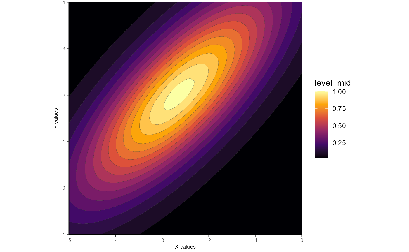

Example 2: Constrained elliptical

As noted above, the constrain_orientation can be used to dictate the orientation. Please note that this will very likely result in a poorer fit, but may be useful for certain types of analyses.

Here we’ll force the Gaussian to be horizontally-oriented.

gauss_fit_ce <-
    fit_gaussian_2D(samp_dat, 
                    constrain_orientation = 0)

gauss_fit_ce
#> Model coefficients
#>   A_o   Amp theta X_peak Y_peak   a    b
#>  1.26 24.77     0  -2.53   1.95 1.2 1.33
#> Model error stats
#>     rss rmse deviance    AIC   R2 R2_adj
#>  885.83 4.96   885.83 231.47 0.54   0.53
#> Fitting methods
#>          method       amplitude     orientation 
#>    "elliptical" "unconstrained"   "constrained"

We’ll use the same grid of x- and y- points as above

## Predict the values using predict_gaussian_2D
gauss_data_ce <-
  predict_gaussian_2D(
    fit_object = gauss_fit_ce,
    X_values = grid$X_values,
    Y_values = grid$Y_values,
  )

## Plot via ggplot2 and metR
ggplot_gaussian_2D(gauss_data_ce)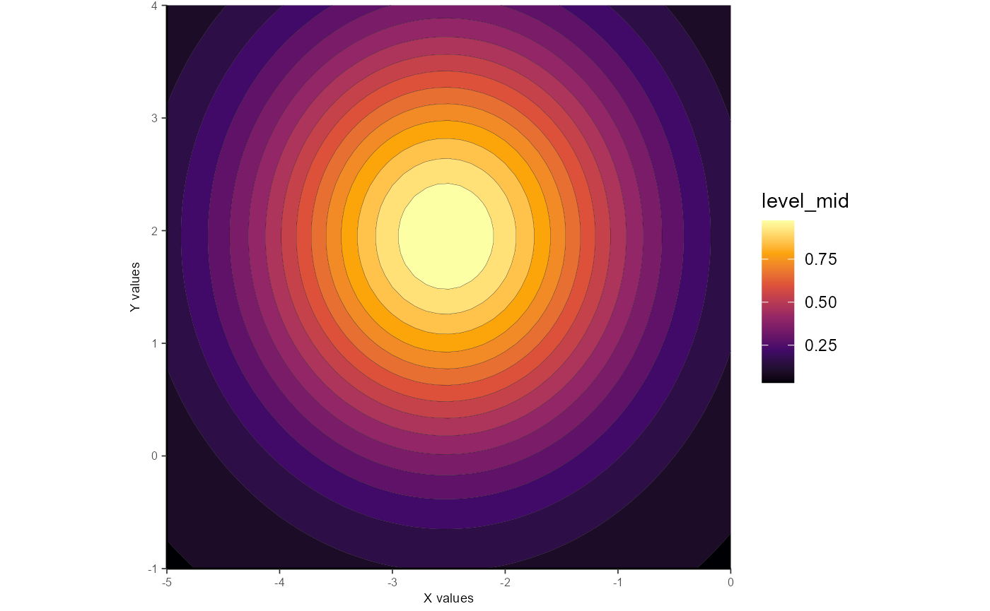

Example 3: Unconstrained elliptical_log

This procedure follows the formula used in Priebe et al. 2003 and is geared towards log2-transformed data (which the example data are).

Parameters from this model include: Amp (amplitude), Q (orientation parameter), X_peak (x-axis peak location), Y_peak (y-axis peak location), X_sig (spread along x-axis), and Y_sig (spread along y-axis).

gauss_fit_uel <-
    fit_gaussian_2D(samp_dat, 
                    method = "elliptical_log")

gauss_fit_uel
#> Model coefficients
#>    Amp     Q X_peak Y_peak X_sig Y_sig
#>  32.23 -0.19  -2.63   2.01  2.11  1.42
#> Model error stats
#>     rss rmse deviance    AIC   R2 R2_adj
#>  169.88 2.17   169.88 172.02 0.92   0.92
#> Fitting methods
#>           method        amplitude      orientation 
#> "elliptical_log"  "unconstrained"  "unconstrained"

## Predict the values using predict_gaussian_2D
gauss_data_uel <-
  predict_gaussian_2D(
    fit_object = gauss_fit_uel,
    X_values = grid$X_values,
    Y_values = grid$Y_values,
  )

## Plot via ggplot2 and metR
ggplot_gaussian_2D(gauss_data_uel)

Example 4: Constrained elliptical_log

Similar to the above, but here the constrain_orientation can be used to dictate the value of the Q parameter used in Priebe et al. 2003. Setting Q to 0 will result in a diagonally-oriented Gaussian, whereas setting Q to -1 will result in horizontal orientation. Q is a continuous parameter, so values in between may be used as well, such as in this example:

gauss_fit_cel <-
    fit_gaussian_2D(
      samp_dat,
      method = "elliptical_log",
      constrain_orientation = -0.66
    )

gauss_fit_cel
#> Model coefficients
#>    Amp     Q X_peak Y_peak X_sig Y_sig
#>  40.37 -0.66   -2.6   2.06  1.85  1.25
#> Model error stats
#>    rss rmse deviance    AIC   R2 R2_adj
#>  406.1 3.36    406.1 201.39 0.81    0.8
#> Fitting methods
#>           method        amplitude      orientation 
#> "elliptical_log"  "unconstrained"    "constrained"

## Predict the values using predict_gaussian_2D
gauss_data_cel <-
  predict_gaussian_2D(
    fit_object = gauss_fit_cel,
    X_values = grid$X_values,
    Y_values = grid$Y_values,
  )

## Plot via ggplot2 and metR
ggplot_gaussian_2D(gauss_data_cel)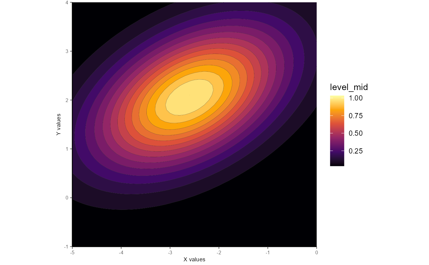

Again, setting the value of Q via constrain_orientation will very likely result in poorer-fitting Gaussians. See the analyses in Priebe et al. 2003 to get a sense of useful applications of this approach. Forcing Q = -0.66 in the above example isn’t all that useful, but goes to show that it can be done.

Example 5: Circular

Using method = "circular" constrains the Gaussian to have a roughly circular shape (i.e. spread in X- and Y- are roughly equal).

If this method is used, the fitted parameters are: Amp (amplitude), X_peak (x-axis peak location), Y_peak (y-axis peak location), X_sig (spread along x-axis), and Y_sig(spread along y-axis).

gauss_fit_cir <-
    fit_gaussian_2D(samp_dat, 
                    method = "circular")

gauss_fit_cir
#> Model coefficients
#>    Amp X_peak Y_peak X_sig Y_sig
#>  23.18  -2.55   1.81  1.32  1.64
#> Model error stats
#>     rss rmse deviance    AIC   R2 R2_adj
#>  899.61    5   899.61 230.03 0.54   0.53
#> Fitting methods
#>          method       amplitude     orientation 
#>      "circular" "unconstrained"              NA

## Predict the values using predict_gaussian_2D
gauss_data_cir <-
  predict_gaussian_2D(
    fit_object = gauss_fit_cir,
    X_values = grid$X_values,
    Y_values = grid$Y_values,
  )

## Plot via ggplot2 and metR
ggplot_gaussian_2D(gauss_data_cir)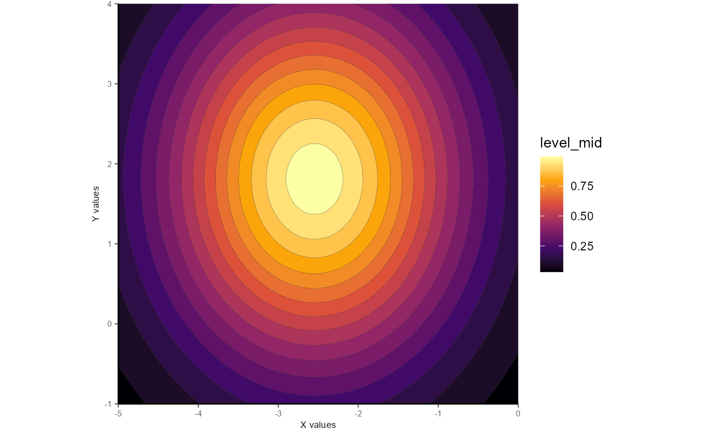

That’s all!

🐢

Priebe NJ, Cassanello CR, Lisberger SG. The neural representation of speed in macaque area MT/V5. J Neurosci. 2003 Jul 2;23(13):5650-61. doi: 10.1523/JNEUROSCI.23-13-05650.2003.↩︎

Vikram B. Baliga

2021-07-29

Overview

The `method` and `constrain_orientation` arguments

`method`

`constrain_orientation`

Example 1: Unconstrained elliptical

Example 2: Constrained elliptical

Example 3: Unconstrained elliptical_log

Example 4: Constrained elliptical_log

Example 5: Circular

Fitting 2D-Gaussians to Data

Vikram B. Baliga

2021-07-29

Overview

The method and constrain_orientation arguments

method

constrain_orientation

Example 1: Unconstrained elliptical

Example 2: Constrained elliptical

Example 3: Unconstrained elliptical_log

Example 4: Constrained elliptical_log

Example 5: Circular

The `method` and `constrain_orientation` arguments

`method`

`constrain_orientation`