
Labs using R: UBC Edition
Lab
5. Describing data
This lab is part of a series designed for BIOL 300, based on The Analysis of Biological Data. The rest of the labs can be found here.
Learning outcomes
Investigate sampling error; see that larger samples have less sampling error.
Visualize confidence intervals.
Calculate basic summary statistics using R.
Calculate confidence intervals for the mean with R.
If you have not already done so, download the
zip file containing Data, R scripts, and other resources for these
labs. Remember to start RStudio from the ABDLabs.Rproj
file in that folder to make these exercises work more seamlessly.
Learning the tools
Missing data
Sometimes we do not have all variables measured on all individuals in
the data set. When this happens, we need a space holder in our data
files so that R knows that the data is missing. The standard way of
doing this in R is to put NA (no quotes) in the location
that the data would have gone. NA is short for “not
available”.
For example, in the Titanic data set, we do not know the age of several passengers. Let’s look at it. Import the Titanic data set:
Have R print out the list of the age variable, which you
can do easily by just typing its name:
If you look through the results, you will see that most individuals
have numbers in this list, but some have NA. These
NAs are the people for which we do not have age
information.
By the way, the titanic.csv file simply has nothing in
the places where there is missing data. When R loaded it, it replaced
the empty spots with NA automatically.
Measures of location
This week we want to use R to give some basic descriptive statistics for numerical data.
mean()
We already saw in lab 1 how to calculate the mean of a vector of data
using mean(). Unfortunately, if there are missing data we
need to tell R how to deal with it.
A (somewhat annoying) quirk of R is that if we try to take the mean
of a list of numbers that include missing data, we get an
NA for the result!
## [1] NAna.rm = TRUE
To get the mean of all the numbers that we do have, we have to add an
option to the mean() function. This option is
na.rm = TRUE.
## [1] 31.19418This tells R to remove (“rm”) the NAs before taking the
mean. It turns out that the mean age of passengers that we have
information for was about 31.2.
na.rm = TRUE can be added to many functions in R,
including median(), as we shall see next.
median()
The median of a series of numbers is the “middle” number – half of
the numbers in the list are greater the median and half are below it. It
can be calculated in R by using median().
## [1] 30summary()
A handy function that will return both the mean and median at the
same time (along with other information such as the first and third
quartiles) is summary().
##    Min. 1st Qu.  Median    Mean 3rd Qu.    Max.     NAs
##  0.1667 21.0000 30.0000 31.1942 41.0000 71.0000     680
From left to right, this output gives us the smallest (minimum) value
in the list (Min.), the first quartile
(1st Qu.), the median, the mean, the third quartile
(3rd Qu.), the largest (maximum) value (Max.),
and finally, the number of individuals with missing values
(NA’s).
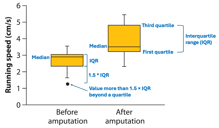
The first quartile is the value in the data that is larger than a quarter of the data points. The third quartile is larger than ¾ of the data. These are also called the 25th percentile and the 75th percentile, respectively. (You may remember these from boxplots, where the top and bottom of the box mark the 75th and 25th percentiles, respectively.)
Measures of variability
R can also calculate measures of the variability of a sample. In this section we’ll learn how to calculate the variance, standard deviation, coefficient of variation and interquartile range of a set of data.
var()
To calculate the sample variance of a list of numbers, use
var().
## [1] 217.4895Note that var(), as well as sd() below,
have the same need for na.rm = TRUE when analyzing data
that include missing values.
sd()
The sample standard deviation can be calculated by
sd().
## [1] 14.74753Of course, the sample standard deviation is the same as the square root of the sample variance.
## [1] 14.74753Coefficient of variation
Surprisingly, there is no standard function in R to calculate the coefficient of variation. You can do this yourself, though, directly from the definition:
## [1] 47.27653IQR()
The interquartile range (or IQR) is the difference between the third
quartile and the first quartile; in other words the range covered by the
middle half of the data. It can be calculated easily with
IQR().
## [1] 20Note that this is the same as we could calculate by the results from
summary() above. The third quartile is 41 and the first
quartile is 21, so the difference is 41 – 21 = 20.
Remember from last week that the IQR is also shown within a boxplot:
Confidence interval of the mean
The confidence interval for an estimate tells us a range of values that is likely to contain the true value of the parameter. For example, in 95% of random samples the 95% confidence interval of the mean will contain the true value of the mean.
R does not have a simple built-in function to calculate only the
confidence interval of the mean, but the function that calculates
t-tests will give us this information. (See chapters 11 and 12
in the text or Labs 8 and 9 for more on t-tests.) The function
t.test() has many results in its output. By adding
$conf.int to this function we only get back the confidence
interval for the mean. By default it gives us the 95% confidence
interval.
## [1] 30.04312 32.34524
## attr(,"conf.level")
## [1] 0.95
As the result above shows, the 95% confidence interval of the mean of
age in the titanicData data set is from about 30.0 to 32.3.
R also tells us that it used a 95% confidence level for its calculation.
(The confidence interval is not so useful in this case, because we
actually have information for nearly all the individuals on the
Titanic.)
To calculate confidence intervals with a different level of
confidence, we can add the argument conf.level to the
t.test() function. For example, for a 99% confidence
interval we can use the following.
## [1] 29.67976 32.70861
## attr(,"conf.level")
## [1] 0.99
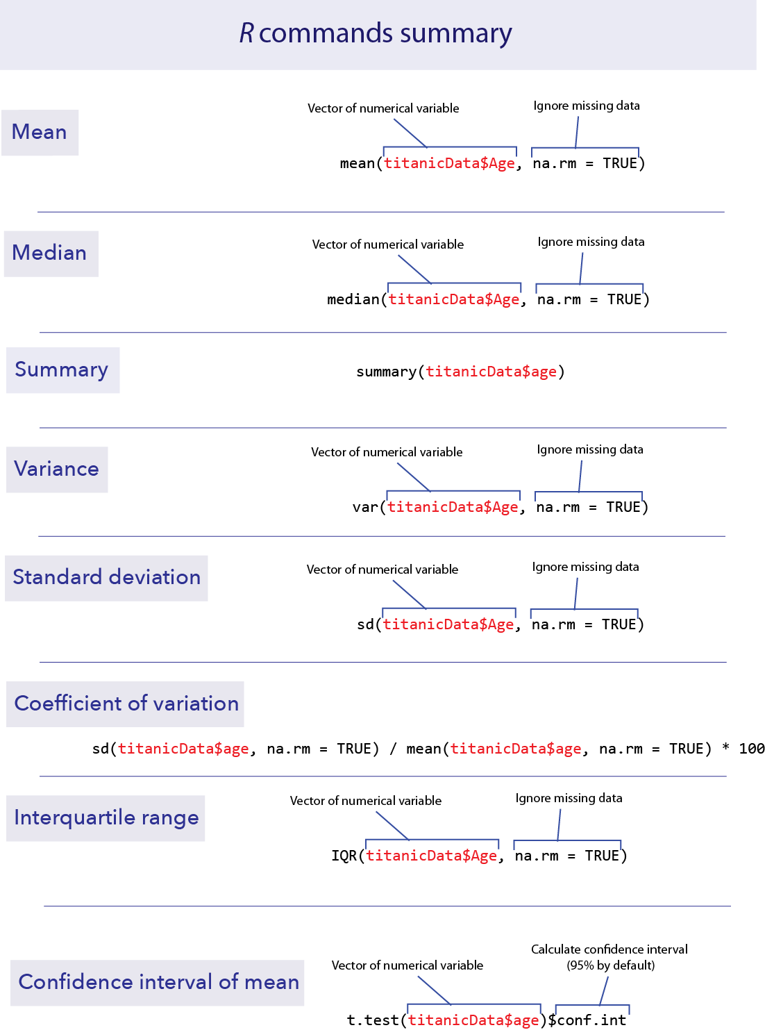
R commands summary
Activities & Questions
Make a script in RStudio that includes all your R code to answer the
following questions. Include answers to all questions below using
comments.
1. Go to the web and open the page at http://www.zoology.ubc.ca/~whitlock/kingfisher/SamplingNormal.htm.
This page contains some interactive visualizations that let you play
around with sampling to see the distribution of sampling means. Click
the button that says “Tutorial” near the bottom of the page and follow
along with the instructions.
In the tutorial, when you were instructed to move the slider for “n” to the right, did the distribution of sample means get wider, narrower, or stay the same compared to when the sample size was 10?
The breadth of the sampling distribution may be affected by one or more sliders. Identify all sliders that seem to affect the breadth of the sampling distribution. Next, identify all sliders that affected the location of the sampling distribution’s center.
What population parameter will the center of the sampling distribution of the mean be equal to?
2. Go back to the web, and open the page at http://www.zoology.ubc.ca/~whitlock/kingfisher/CIMean.htm
. This applet draws confidence intervals for the mean of a known
population. Click “Tutorial” again, and follow along.
What does the word “failure” mean in the context of this tutorial?
When you switched to using a 99% confidence interval, did the intervals get wider, narrower, or stay the same?
3. In Lab 4, we used a data set of all recorded measurements
from Lab 1 from all BIOL 300 students. Import that data set into R again
(see Canvas if you need to download it again). Remember that these data
were collected using measuring tapes based in inches, but the activity
asked for the measurements in centimenters.
- Plot the distribution of height in the class. Describe the shape of the distribution. Is it symmetric or strongly skewed? Is it unimodal or bimodal? Then do the same for the distribution of head circumference and for arm span. Is it symmetric and unimodal?
Key point: A distribution is skewed if it is asymmetric. A
distribution is skewed right if there is a long tail to the right, and
skewed left if there is a long tail to the left. 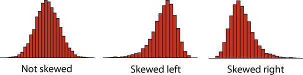
For any of these 3 variables (height, head circumference, arm span), are there any large outliers that look as though a student used the wrong units for their measurement? (E.g., more plausibly a height recorded in inches rather than the requested centimeters?) If so, and if this is not likely to be an accurate description of an individual in your class, use
filter()to create a new data set without those rows. The best practice would be to do this separately for each variable. Filtering out all rows withNAs could risk throwing out reasonable measurements from cells that do not haveNA.Use R to calculate the mean of each of the 3 variables, using each filtered dataset if necessary for each variable.
Calculate the standard deviation of each of the 3 variables, using each filtered dataset if necessary for each variable.
4. The file caffeine.csv contains data on the
amount of caffeine in a 16 oz. cup of coffee obtained from various
vendors. For context, doses of caffeine over 25 mg are enough to
increase anxiety in some people, and doses over 300 to 360 mg are enough
to significantly increase heart rate in most people. A can of Red Bull
contains 80mg of caffeine.
What is the mean amount of caffeine in 16 oz. coffees?
What is the 95% confidence interval for the mean?
Plot the frequency distribution of caffeine levels for these data in a histogram. Is the amount of caffeine in a cup of coffee relatively consistent from one vendor to another? What is the standard deviation of caffeine level? What is the coefficient of variation?
The file
caffeineStarbucks.csvhas data on six 16 oz. cups of Breakfast Blend coffee sampled on six different days from a Starbucks location. Calculate the mean (and the 95% confidence interval for the mean) for these data. Compare these results to the data taken on the broader sample of vendors in the first file. Describe the difference.
5. A confidence interval is a range of values that are likely to
contain the true value of a parameter. Consider the
caffeine.csv data again.
- Fix any mistakes in the code below to calculate the 99% confidence interval for the mean caffeine level.
Compare this 99% confidence interval to the 95% confidence interval you calculate in question 4b. Which confidence interval is wider (i.e., spans a broader range)? Why should this one be wider?
Let’s compare the quantiles of the distribution of caffeine to this confidence interval. Approximately 95% of the data values should fall between the 2.5% and 97.5% quantiles of the distribution of caffeine. (Explain why this is true.) We can use R to calculate the 2.5% and 97.5% quantiles with a line like the following. (Replace
datavectorwith the name of the vector of your caffeine data.)
Are these the same as the boundaries of the 95% confidence interval? If not, why not? Which should bound a smaller region, the quantile or the confidence interval of the mean?
6. Return to our class data set. Find the mean value of “number
of siblings”. Add 1 to this to find the mean number of children per
family in the class.
The mean number of offspring per family a few decades ago was about 2. Is the value for this class similar, greater, or smaller? If different, think of reasons for the difference.
Are the families represented in this class systematically different from the population at large? Is there a potential sampling bias?
Consider the way in which the data were collected. How many families with 0 children are represented? Why? What effect does this have on the estimated mean family size of all couples?
7. Return to the data on countries of the world, in
countries.csv. Plot the distributions for
ecological_footprint_2000,
cell_phone_subscriptions_per_100_people_2012, and
life_expectancy_at_birth_female.
For each variable, plot a histogram of the distribution. Is the variable skewed? If so, in which direction?
For each variable, calculate the mean and median. Are they similar? Match the difference in mean and median to the direction of skew on the histogram. Do you see a pattern?
Last substantive update: 2026-08-21