
Labs using R: UBC Edition
Lab
6. Frequency data
This lab is part of a series designed for BIOL 300, based on The Analysis of Biological Data. The rest of the labs can be found here.
Learning outcomes
Calculate a confidence interval for a proportion
Make a hypothesis test about proportions.
Fit frequency data to a model.
Test for a fit to a Poisson distribution.
If you have not already done so, download the
zip file containing Data, R scripts, and other resources for these
labs. Remember to start RStudio from the ABDLabs.Rproj
file in that folder to make these exercises work more seamlessly.
Learning the tools
Confidence interval for a proportion
To calculate a confidence interval for an estimate of a proportion,
we suggest using the Agresti-Coull method. This method is available in
the R package binom, which you can install and load with
the following:
Like any package, you only need to install it once, but you need to run the library command in each session before you can use it.
Once the package is installed, calculating a confidence interval for
a proportion is fairly straightforward. The function you need is called
binom.confint(). You need to specify:
x: the number of successesn: the total sample sizemethod = "ac"for Agresti-Coull
For example, if we have 87 data points and 30 of them are “successes”, we can find the 95% confidence interval for the proportion of successes with the following command.
##          method  x  n      mean     lower     upper
## 1 agresti-coull 30 87 0.3448276 0.2532164 0.4495625
This tells us that the observed proportion (called mean
here) is 0.3448, and the lower and upper bounds of the 95% confidence
interval are 0.2532 and 0.4496.
For more details, see the Help page by running
?binom.confint in the Console.
Binomial tests
Doing a binomial test in R is much easier than doing one by hand.
binom.test()
The function binom.test() will do an exact binomial
test. It requires three pieces of information in the input:
xfor the number of “successes” observed in the datanfor the total number of datapfor the proportion given by the null hypothesis
For example, if we have 18 toads that have been measured for a
left-right preference and 14 are right-handed, we can test the null
hypothesis of equal probabilities of left- and right-handedness with a
binomial test. (See Example 6.2 in the text.) In this case,
x = 14, n = 18, and p = 0.5.
##
##  Exact binomial test
##
## data:  14 and 18
## number of successes = 14, number of trials = 18, p-value = 0.03088
## alternative hypothesis: true probability of success is not equal to 0.5
## 95 percent confidence interval:
##  0.5236272 0.9359080
## sample estimates:
## probability of success
##              0.7777778
In this case, the output of the function gives quite a bit of information. One key element that we will be looking for is the P-value; in this case R tells us that the P-value is 0.03088. This is the P-value that corresponds to a two-tailed test.
The binom.test() function also gives an estimate of the
proportion of successes (in this case 0.7777778). (It also gives an
approximate 95% confidence interval for the proportion using a
different method than the Agresti-Coull method that we
recommend.)
Goodness of fit test
A \(\chi^2\) goodness-of-fit test
compares the frequencies of values of a categorical variable to the
frequencies predicted by a null hypothesis. For example, the file
MandMlist.csv contains a list of all the colors of M&M
candies from one package, under the variable color. Let’s
ask whether this fits the proportions of colors advertised by the candy
company.
MMlist$color contains the color of each of 55
M&Ms.
table()
Summarizing frequency data in a table is useful to see the data more
concisely, and such a table is also necessary as input to the \(\chi^2\) test function. We can summarize
the counts (frequencies) of a categorical variable with
table().
##
##   blue  brown  green orange    red yellow
##     10      5     12     11      6     11
This shows that in this list of M&M colors, 10 were blue, 5 were brown, etc.
chisq.test()
We can use a \(\chi^2\)
goodness-of-fit test to compare the frequencies in a set of data to a
null hypothesis that specifies the probabilities of each category. In R,
this can be calculated using the function chisq.test().
The company says that the percentages are 24% blue, 14% brown, 16% green, 20% orange, 13% red and 13% yellow. This is our null hypothesis. Let’s test whether these proportions are consistent with the frequencies of the colors in this bag. R wants the proportions expected by the null hypothesis in a vector, like this:
Notice that R wants you to input the expected proportions, which it will use to calculate the expected frequencies.
The first thing we need to do is check whether the expected frequencies (expected by the null hypothesis) are large enough to justify using a \(\chi^2\) goodness of fit test. (In other words, that no more than 25% of the expected frequencies are less than 5 and none is less than 1.)
To obtain these expected counts, multiply the vector of the expected
proportions by the total sample size. We can find the total sample size
by taking the sum() of the frequency table:
## [1] 55So for this example, the expected frequencies from our null hypothesis are 55 times the list of expected proportions:
## [1] 13.20 7.70 8.80 11.00 7.15 7.15All of these expected values are greater than 5, so we have no problem with the assumptions of the \(\chi^2\) goodness of fit test. (If there were a problem here, we’d have to combine categories. We’ll see an example of that in the next section.)
The function chisq.test() requires two arguments in its
input: a frequency table from the data and a vector with the expected
proportions from the null hypothesis. The name of the vector of expected
proportions in this function is p. So here is the format of
the R command to do a \(\chi^2\)
test:
##
##  Chi-squared test for given probabilities
##
## data:  MMtable
## X-squared = 5.1442, df = 5, p-value = 0.3985
“X–squared” here in the output means \(\chi^2\). The \(\chi^2\) value for this test is 5.1442. There are 5 degrees of freedom (df) for this test, and the P-value turned out to be 0.3985. We wouldn’t reject the null hypothesis with these data.
Fit to a Poisson distribution
A \(\chi^2\) goodness of fit test can be used to ask whether a frequency distribution of a variable is consistent with a Poisson distribution. This is a useful way to determine if events in space or time are not “random” but instead are clumped or dispersed.
It turns out that this is not a straightforward process in R. In this section, we’ll highlight a couple of functions in R that will streamline doing the calculations by hand. We’ll use the data on the numbers of extinctions per prehistoric time period described in Example 8.4 in the Whitlock and Schluter textbook.
extinctData <-
  read.csv("DataForLabs/MassExtinctions.csv",
    stringsAsFactors = TRUE
  )

number_of_extinctions <- extinctData$numberOfExtinctions

table(number_of_extinctions)
## number_of_extinctions
## 1 2 3 4 5 6 7 8 9 10 11 14 16 20
## 13 15 16 7 10 4 2 1 2 1 1 1 2 1The first row lists each possible number of extinctions in a time period, ranging from 1 to 20. The second row shows the number of time periods that had each number of extinctions. (so there were 13 time periods with one extinction, 15 time periods with 2 extinctions, etc.)
The mean number of extinctions per unit of time is not specified by the null hypothesis, so we need to estimate it from the data. This mean turns out to be 4.21 extinctions per time period.
## [1] 4.210526We can use this mean to calculate the probability according to a Poisson distribution of getting each specific number of extinctions.
dpois()
Fortunately, R has a function to calculate the probability of a given
value under the Poisson distribution. This function is
dpois(), which stands for “density of the Poisson”.
dpois() requires two values for input, the mean (which is
called lambda in this function) and x, the
value of the outcome we are interested in (here, the number of
extinctions). For example, the probability of getting x = 3
from a Poisson distribution with mean 4.21 can be found from the
following:
## [1] 0.1846076The probability of getting exactly 3 successes from a Poisson distribution with mean 4.21 is about 18.5%.
dpois() will accept a vector of x’s as
input, and return a vector of the probabilities of those
xs. A convenient short hand to know here is that R will
create a vector with a range of values with a colon. For example, 0:19
is a vector with the integers from 0 to 19.
## [1] 0 1 2 3 4 5 6 7 8 9 10 11 12 13 14 15 16 17 18 19This can be plugged directly into dpois() along with the
appropriate lambda to generate the probabilities for the
integers from 0 to 19.
##  [1] 1.483856e-02 6.247813e-02 1.315329e-01 1.846076e-01 1.943238e-01
##  [6] 1.636411e-01 1.148358e-01 6.907419e-02 3.635484e-02 1.700811e-02
## [11] 7.161310e-03 2.741171e-03 9.618145e-04 3.115189e-04 9.368989e-05
## [16] 2.629892e-05 6.920767e-06 1.714122e-06 4.009642e-07 8.885633e-08
We’ll need the probabilities for all possible values of ‘x’ we see in the data, but recall that the Poisson distribution extends from 0 to infinity. To get the probability for x ≥ 20, we can keep in mind that that the sum of all probabilities must equal 1. We can therefore create a vector with the Poisson probabilities of each possibility from 0 to 20 like this:
expected_0to19 <- dpois(x = 0:19, lambda = mu)
expected_probability <- c(expected_0to19, 1 - sum(expected_0to19))
expected_probability
## [1] 1.483856e-02 6.247813e-02 1.315329e-01 1.846076e-01 1.943238e-01
## [6] 1.636411e-01 1.148358e-01 6.907419e-02 3.635484e-02 1.700811e-02
## [11] 7.161310e-03 2.741171e-03 9.618145e-04 3.115189e-04 9.368989e-05
## [16] 2.629892e-05 6.920767e-06 1.714122e-06 4.009642e-07 8.885633e-08
## [21] 2.333422e-08The odd notation here is a shorthand for scientific notation. 1.48e-02 means 1.48 x 10⁻². The e stands for exponent.
Remember that we asked R to output the probability of values from 0 to 20+. Consequently, there are 21 numbers listed. The first value in this output corresponds to the probability of getting a zero, the second to the probability of getting a 1, etc. The 21st value (2.328750e-08) corresponds to the probability of x ≥ 20 (i.e., all the way out to infinity).
In order to convert these probabilities into expected values for a \(\chi^2\) test, we need to multiply them by the total sample size.
##  [1] 1.127730e+00 4.748338e+00 9.996501e+00 1.403018e+01 1.476861e+01
##  [6] 1.243672e+01 8.727524e+00 5.249639e+00 2.762968e+00 1.292616e+00
## [11] 5.442596e-01 2.083290e-01 7.309790e-02 2.367543e-02 7.120431e-03
## [16] 1.998718e-03 5.259783e-04 1.302733e-04 3.047328e-05 6.753081e-06
## [21] 1.773401e-06
Most of these values would cause problems for the \(\chi^2\) test because they are too small (less than 1). We need to combine categories in some reasonable way so that the expected frequencies match the assumptions of the \(\chi^2\) test. Let’s combine the categories for 0 and 1 successes, and combine everything greater than or equal to 8 into one category. It is possible to do this all in R, but you can also do it by hand, using the expected frequencies we just calculated.
Here’s how you can do it in R, using the c() function
and indexing. Note that the sum() function is used to
combine wherever needed. The colon (:) means “through”.
E.g., 9:21 means “9 through 21”.
expected_combined <-
  c(sum(expected_values[1:2]), # 0 or 1
    expected_values[3:8],      # 2 through 7
    sum(expected_values[9:21]) # 8 or more
  )
expected_combined
## [1] 5.876068 9.996501 14.030177 14.768608 12.436722 8.727524 5.249639
## [8] 4.914761Here is a table of the expected frequencies for these new combined categories, for both the observed and expected, summing over all the possibilities within each of these groupings. (E.g., the expected frequency for the category “0 or 1” is the sum of 1.128324 and 4.750244.)
| Number of extinctions | Expected | Observed |
|---|---|---|
| 0 or 1 | 5.876068 | 13 |
| 2 | 9.996501 | 15 |
| 3 | 14.030177 | 16 |
| 4 | 14.768608 | 7 |
| 5 | 12.436722 | 10 |
| 6 | 8.727524 | 4 |
| 7 | 5.249639 | 2 |
| 8 or more | 4.914761 | 9 |
Note that these expected values are large enough to match the conditions of the \(\chi^2\) test.
Make vectors, using c(), for the observed and expected
values for these new groups. If you didn’t use the R code to make
expected_combined automatically from the
expected_values object, the code below can be used.
expected_combined <-
  c(5.876068, 9.996501, 14.030177, 14.768608,
    12.436722, 8.727524, 5.249639, 4.914761)

observed_combined <- c(13, 15, 16, 7, 10, 4, 2, 9)
From these we can calculate the \(\chi^2\) test statistic using
chisq.test()$statistic.
We give it first the list of observed values, then the expected
values as p. Because we are giving the list of expected
frequencies rather the expected probabilities, we need to give it the
option rescale.p = TRUE. Finally, by adding
$statistic at the end, R will only give us the \(\chi^2\) value as output. (We don’t yet
want the full results of the test because R does not know to correct for
the reduction in degrees of freedom caused by estimating the mean.)
## Warning in chisq.test(observed_combined, p = expected_combined, rescale.p
## = TRUE): Chi-squared approximation may be incorrect## X-squared
## 23.94974This correctly calculates our \(\chi^2\) value as 23.94974. The warning message is because one of the expected values is under 5, but because this occurred in less than 20% of the categories, it is fine to proceed.
The degrees of freedom for this test are the number of categories minus the number of parameters estimated from the data minus one. We ended up using 8 categories and estimated one parameter from the data, so we have df = 8 – 1 – 1 = 6.
pchisq()
To calculate the correct P-value, we need to know
probability of getting a \(\chi^2\)
value greater than 23.94974 from a distribution that has 6 degrees of
freedom. R has a function we can use for this, called
pchisq(). We are interested here in the probability above
the observed \(\chi^2\) value, so we
want the probability in the right (or upper) tail. To use this function,
we need to specify three values: our observed \(\chi^2\) (confusingly called q
in this function), the degrees of freedom (called df, thank
goodness), and an option that tells us to use the upper tail
(lower.tail = FALSE).
##    X-squared
## 0.0005334917
Thus, our P-value for this test of the fit of these data to a Poisson distribution is approximately 0.0005. We reject the null hypothesis that these extinction data follow a Poisson distribution.
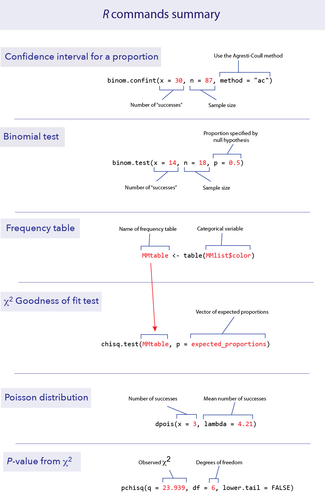
R commands summary
Activities & Questions
Make a script in RStudio that includes all your R code to answer the
following questions. Include answers to all questions below using
comments.
1. This is a simple, quick exercise meant to help you visualize
the meaning of a binomial distribution. The binomial distribution
applies to cases where we do a set number of random trials, and in each
trial there is an equal and independent probability of a success. Let’s
say there are n trials and the probability of success is
p. Of those n trials, anywhere between 0 and n of them
could be a ’success” and the rest will be “failures.” Let’s call the
number of successes X.
As our example, let’s roll five regular dice, and keep track of how many come up as “three.” In this case, there are five trials, so n = 5. The probability of rolling a “three” is 1/6, so p = 0.1666.
Let’s repeat the sampling process a lot of times. For each sample, roll five dice, and record the number of threes.
(If you don’t have dice available, you can simulate rolling dice at https://shiney.zoology.ubc.ca/otto/Dice/)
For this exercise, draw a histogram of the results by hand. First draw the axes, and then for each result draw an X stacked up in the appropriate place. For example, after three trials that got 0, 1, and 1 threes, respectively, the histogram will look like this:
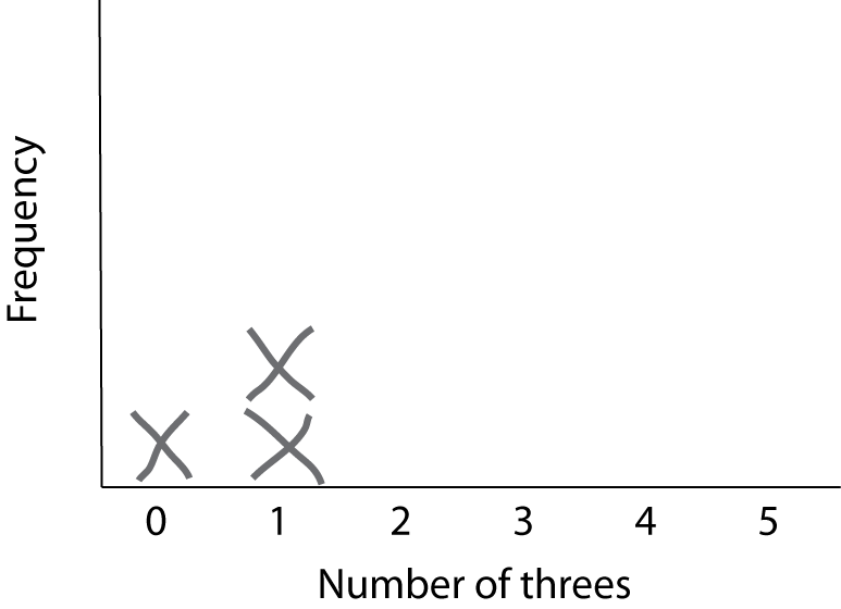
Keep doing this until you have 20 or more samples.
Here is the frequency distribution for this process as calculated from the binomial distribution.
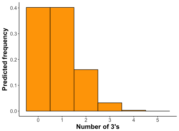
Is this similar to what you found? (Remember that with only a few trials, you don’t expect to exactly match the predicted distribution. If you increase your number of samples, the fit should improve.)
- The expected mean number of threes is 0.833. (For the binomial
distribution, the mean is
n×p, or in this case 5 × 0.1666.) Calculate the mean number of threes in your samples.
2. Many hospitals still have signs posted everywhere banning
cell phone use. These bans originated from studies on earlier versions
of cell phones. In one such experiment, out of 510 tests with cell
phones operating at near-maximum power, six disrupted a piece of medical
equipment enough to hinder interpretation of data or cause equipment to
malfunction. A more recent study found zero instances of disruption of
medical equipment out of 300 tests.
For the older data, use
binom.confint()with the Agresti-Coull method to calculate the estimated proportion of equipment disruption. What is the 95% confidence interval for this proportion?For the data on the newer cell phones, use R to calculate the estimate of the proportion and its 95% confidence interval.
3. It is difficult to tell what other people are thinking, and
it may even be impossible to find out what they are thinking by asking
them. A series of studies shows that we do not always know how our own
thought processes are carried out.
A classic experiment by Wilson and Nisbett (1978) addressed this issue in a clever way. Participants were asked to decide which of four pairs of silk stockings were better, but the four stockings that they were shown side-by-side were in fact identical. Nearly all participants were able, however, to offer reasons that they had chosen one pair over the other.
The four pairs of stockings were presented to the participants
randomly with respect to which pair was in which position. However, of
the 52 subjects who selected a pair of stockings, 6 chose the pair on
the far left, 9 chose the pair in the left-middle, 16 chose the pair in
the right-middle, and 21 chose the pair on the far right. None admitted
later that the position had any role in their selection. These data are
in a file called stockings.csv.
- What are the expected frequencies for this scenario, under the null hypothesis that all four pairs of stockings are equally likely to be chosen? Save these frequencies in a vector in R by editing the line below:
Use
chisq.test()to test the null hypothesis that the selection of the stockings was independent of position.The function
chisq.test()can take the data either as a data frame, as above, or as a vector of the observed counts, as a parameter calledxas input:
Try it using the specification of the counts, to see whether you get
the same answer as in (b). The exp_freqs object comes from
your answer to (a).
4. Many people believe that the month in which a person is born
predicts significant attributes of that person in later life. Such
astrological beliefs have little scientific support, but are there
circumstances in which birth month can have a strong effect on later
life? One prediction is that elite athletes will disproportionately have
been born in the months just after the age cutoff used to separate
levels for young players of the sport. The prediction is that those
athletes that are oldest within an age group will do better by being
relatively older, and therefore will gain more confidence and attract
more coaching attention than the relatively younger players in their
same groups. As a result, they may be more likely to dedicate themselves
to the sport and do well later. In the case of soccer, the cutoff for
different age groups is generally August.
The birth months (by three month interval) of soccer players competing in the Under-20’s World Tournament are recorded in the data file
soccer_birth_quarter.csv(from Barnsley et al. 1992). Plot these data. Do you see a pattern?The numbers of people born in Canada by month is recorded in the file
Canadian_births.csv. Compare the distribution of birth months of the soccer players to what would be expected by chance, assuming that the birth data for Canada is a good approximation for the population from which soccer players are drawn. Use the appropriate statistical test. Describe the pattern.
5. Are cardiac arrests (or “heart attacks”) equally likely to
occur throughout the year? Or are some weeks more likely than others to
produce heart attacks? One way to look at this issue is to ask whether
heart attacks occur according to a probability model in which such
events are independent of each other and equally likely at all times. If
so, then the number of heart attacks per week will follow a Poisson
distribution. The data file
cardiac arrests out of hospital.csv contains data on the
number of heart attacks per week from one hospital over five years. It
records the number of heart attacks that occurred to individuals outside
of the hospital who were then brought in for treatment (from Skogvoll
and Lindqvist 1999).
Calculate a table of the observed frequencies of heart attacks per week.
What is the mean number of heart attacks per week?
For the mean you just calculated, use
dpois()to calculate the probability of 0 heart attacks in a week assuming a Poisson distribution. Multiply that probability by the number of data points to calculate the expected frequency of 0 in these data under the null hypothesis of a Poisson distribution.Here is a table of the expected frequencies under the null hypothesis. (The expected frequency for zero heart attacks should match your calculation above.) Are these frequencies acceptable for use in a \(\chi^2\) goodness of fit test?
| Number of heart attacks | Expected |
|---|---|
| 0 | 34.785295 |
| 1 | 70.103698 |
| 2 | 70.640891 |
| 3 | 47.454800 |
| 4 | 23.909219 |
| 5 | 9.636973 |
| 6 or more | 4.469124 |
Create vectors in R for the observed and expected frequencies.
Calculate the \(\chi^2\) for this hypothesis test, using
chisq.test()$statistic.How many degrees of freedom should this \(\chi^2\) goodness of fit test have?
Calculate the P-value for this test using R.
Summarize the results of this test. Does the frequency distribution of out-of-hospital cardiac events follow a Poisson distribution?
Last substantive update: 2026-08-21